Why Does Deep Learning Work So Well ? — From the Physics Standpoint

This blog post is essentially about the gist of the research paper “why does deep and cheap learning work so well?” This paper explores why deep learning (DL) works so well and they have argued that the answer may not only lie in computer science and mathematics, but also in physics. Neural networks (neural nets or NNs) are the foundation of deep learning and they usually outperform virtually every machine learning algorithm out there. One major disadvantage, however, about neural nets is that they don’t exactly show how they get the results that they do. Neural nets have been a major success at tasks such as identifying objects in images, but how they do so remains a mystery. Their exact computations are cloaked from our eyes, which makes it harder to detect errors or biases that they have. This is a problem when neural nets are, for instance, used to decide whether a person should get a loan or not, because if their loan application is denied they will want to know why or at least it should be known why that person was denied by an AI model powered by a neural net. Furthermore, it is important to understand why deep learning works so well so that the learning process can be made faster with less resources and DL models can be made to be more robust. A robust DL model wouldn’t get confused or tricked into outputting an image caption saying that a person in a picture is a lion or something else entirely different than what is expected. Also, deep learning would be useful everywhere just as electricity is. Andrew Ng said
“I think that AI is the new electricity. Starting about 100 years ago, the electrification of our society transformed every major industry. Ranging from transportation, manufacturing, to healthcare, to communications and many more. And today, we see a surprisingly clear path for AI to bring about an equally big transformation. And of course, the part of AI that is rising rapidly and driving a lot of these developments, is deep learning.”
Introduction
In simple terms, a feed forward neural network in deep learning is just a function f(x) where you input something in an input layer and then something comes out:

This something could be data, bits, vectors etc. In fact, in deep learning convolutional neural networks (CNNs), which I wrote blog posts about, are actually feed forward functions. For instance, an input could be an image of a cat or dog that’s fed to a CNN and the output could be the caption of whether it’s a cat or dog image. Deep learning is essentially about approximating functions, in particular, probability distributions.

If you are trying to predict model parameters y given the data x, then it’s called classification. In other words, classification is when you know what the output is, but you are trying to predict what the input is. For example, if you have a pic of a famous person as an output but you’re trying to predict their name, then it’s classification. If however, you are trying to predict the data x given the model parameters y, then that’s called generation (or prediction). For example, if you type an email and you are trying to predict what word(s) to type next, then that’s called generation. This can be done with natural language processing, by the way. Sometimes we just want to find the probability itself, without any assumptions or beliefs of the causality of x and y , i.e we just have the data x itself and we are trying to find the patterns from the data and see what probability distribution is the data drawn from, we call that unsupervised learning.
There’s a well-known mathematical theorem such as the Stone–Weierstrass theorem from mathematical analysis, which essentially says that polynomials can approximate any function arbitrarily well (i.e as well as desired). As a consequence, there is a Universal Approximation Theorem which basically says that a neural network can approximate any continuous function, provided it has at least one hidden layer and uses non-linear activations there. So, according to mathematics, it shouldn’t be very surprising that neural networks can work so well if they are made arbitrarily bigger.
Why is it Surprising That Deep Learning Works so Well?

If you have let’s say a convolutional neural network that can take say a 1000 by 1000 gray scale image (that is, a one megapixel black and white image), how many pictures can you possibly input into your convolutional neural network? Well, the answer to that is 2¹ ⁰⁰⁰ ⁰⁰⁰ images, as it turns out, that’s more images than there are particles in the universe; 10⁸⁶ particles. So, if we want to compute the probability that whether a gray-scaled 1000 by 1000 image is an image of a cat or dog, it means that for each image there must be 2¹ ⁰⁰⁰ ⁰⁰⁰ parameters stored, i.e 2¹ ⁰⁰⁰ ⁰⁰⁰ probabilities. So, one might expect that this all means that doing good image recognition with a convolutional neural network is impossible, but that’s not the case.
So basically here’s what happens: the neural networks perform a combinatorial “swindle,” replacing exponentiation by multiplication — if there are say 10⁶ inputs taking 2 values each, this swindle cuts the number of parameters from 2¹ ⁰⁰⁰ ⁰⁰⁰ to 2 * 10⁶ times some constant factor. As the authors showed in the paper, “the success of this swindle depends fundamentally on physics: although neural networks only work well for an exponentially tiny fraction of all possible inputs, the laws of physics are such that the data sets we care about for machine learning (natural images, sounds, drawings, text, etc.) are also drawn from an exponentially tiny fraction of all imaginable data sets.”
This basically means that the images that we care about are special images that do not at all look like images that which are randomly generated. Actually, a randomly generated image with a million pixels doesn’t look very different from pure noise. This has actually been proved by the mathematician Émile Borel.
Connection to Physics
Since Hamiltonians in physics have properties that make them easier to evaluate, the authors used this to their advantage by simply rewriting the Bayes’ Theorem (1) in terms of the well-known Hamiltonian H (2) to get it in the form (3):

NB: the negative logs were introduced in order to substitute in the Hamiltonian H, hence that’s why the exponential function has a negative sign.
As it turns out, “the Hamiltonians that show up in physics are not random functions, but tend to be polynomials of very low order, typically of degree ranging from 2 to 4,” as the authors wrote. Also thanks to the Central Limit Theorem (CLT), many probability distributions in machine learning and statistics are approximated by multi-variate distributions of the form

which means that the Hamiltonian H = -ln p is a quadratic polynomial.
In physics, locality is the principle stating that an object is directly influenced only by its immediate surroundings. Also, in general, “ there are certainly cases in physics where locality is still approximately preserved, for example in the simple block-spin renormalization group, spins are grouped into blocks, which are then treated as random variables. To a high degree of accuracy, these blocks are only coupled to their nearest neighbors. Such locality is famously exploited by both biological and artificial visual systems, whose first neuronal layer performs merely fairly local operations.”
One other important point that the authors make is about symmetry: whenever the Hamiltonian obeys some symmetry (is invariant under some transformation), the number of independent parameters required to describe it is further reduced. For instance, many probability distributions in both physics and machine learning are invariant under translation and rotation.
Symmetry reduces not just the the number of parameters but also the computational complexity. For example, if a linear vector-valued function f(x) mapping a set of n variables onto itself happens to satisfy translational symmetry, then it is a convolution (implementable by a convolutional neural net), which means that it can be computed with n log₂ (n) rather than n² multiplications using Fast Fourier transform.
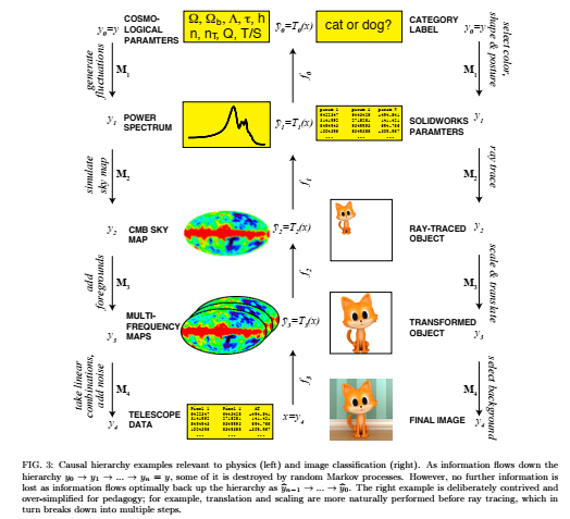
When it comes to connecting physics to deep learning, we would have to turn to renormalization. In simple terms, renormalization in physics is really just a process of figuring out what information do we care about and getting rid of things that we don’t care about. Renormalization is analogous to the process of analyzing data in deep learning, as shown in fig.3 below, where features are extracted and the noise is thrown away.

The Gist
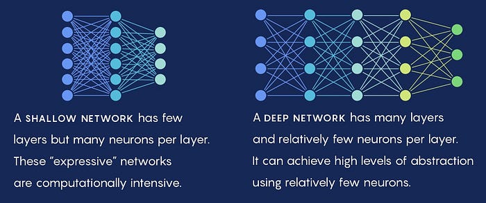
Shallow neural networks rely on symmetry, locality and polynomial log-probability which favors low-order Hamiltonians that the paper presented. They conclude that their arguments are relevant in explaining why there has been a success in applying machine learning techniques to physics. When it comes to deep learning, they essentially proved that there are much less neurons needed by a deep neural network than in a shallow neural network with just one hidden layer; which means that flattening a neural network with multiple hidden layers to a neural network with just one hidden layer means that there would be a loss in efficiency (which is the measure of the number of neurons or parameters that the neural network requires to approximate a given function). In particular, there are 2^n neurons needed to multiply n numbers with a shallow neural network with one hidden layer, whereas they showed that there are 4n neurons needed with a deep network. So basically what this means is that to multiply 20 numbers, there are at least 2²⁰ = 1,048,576 neurons needed in a neural network with one hidden layer compared to just 4 * 20 = 80 neurons that are needed in a deep neural network. What that means, pictorially below, is that far more neurons in a hidden layer are actually needed for the simple neural network on the left than in a deep neutral network on the right, just to even multiply 20 numbers.

In summary, nature gives us probability distributions of images and sounds of a special kind (which are not like randomly generated images or sounds etc) and it turns out that neural nets are good at approximating almost no functions, but neural nets are good at approximating this very special kind of images, that we care about in nature (such as an image of a dog, person, car etc).
Other Resources
These are just a couple of resources that I found to be useful for further reading.
